Feature guide · Scopes
Scopes — see the sound, not just react to it.
Four instrument-style visualizers built into Spiralyst Lab — a true oscilloscope, an X-Y vectorscope, a frequency spectrum analyzer, and a parametric harmonograph. Where the fractals are audio-reactive art, the scopes are audio visualization: instruments that show you the sound itself.
From reacting to revealing
For the 27 fractal forms in Spiralyst Lab, sound is fuel — the bass pushes the zoom, the hats shimmer the color, the lead bends the geometry. The picture is the art and the audio drives it. Scopes turn that gaze around. They keep the same canvas, the same color and effects controls, the same recording and export, but what they draw is the audio itself — its waveform, its stereo image, its frequency content, or the mathematical curve that audio could be made to dance.
That makes scopes useful in different rooms. A math educator can project the spectrum and walk students through Fourier's idea — that any sound is a sum of sines — while a track plays. A DJ or live engineer can pull up the Lissajous to check that a mix sums to mono cleanly. A hobbyist can leave the oscilloscope running with their favorite album and watch the shape of every instrument live. And a curious student can spend an afternoon with the harmonograph, learning how two coupled oscillations make every spirograph pattern ever drawn.
The four modes
Oscilloscope — the waveform
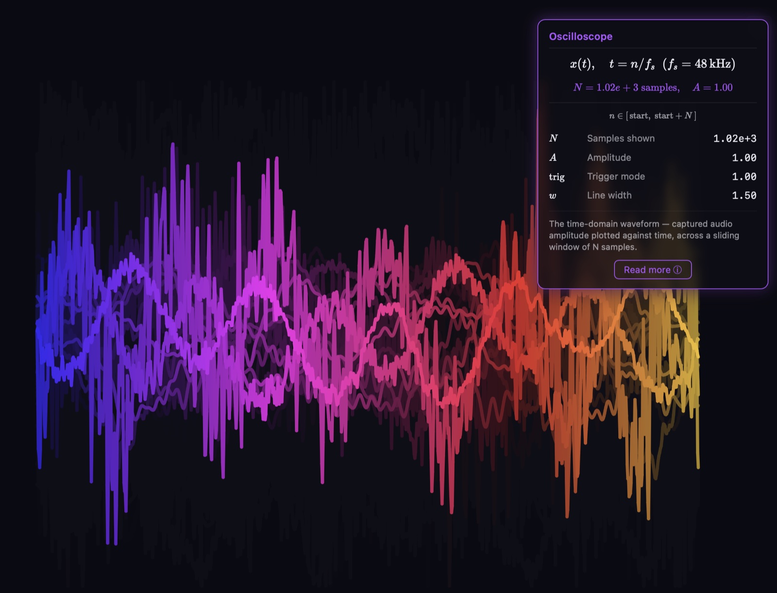
x(t), t = n/fₛ alongside the live waveform.
The classic. An oscilloscope plots the audio waveform directly: time across the screen, amplitude up and down. It's the most direct picture of a sound there is — a moving graph of exactly what the speaker cone is doing, instant by instant. Spiralyst Lab's oscilloscope is a true software oscilloscope of the captured audio, not a stylized approximation.
The trace is the signal itself:
$$x(t),\quad t = \frac{n}{f_s}$$
where \(x\) is the sample value, \(n\) is the sample number, and \(f_s\) is the sample rate. With a 48 kHz capture, sample number 1 sits at \(t = 1/48{,}000\) seconds. Only a short window of samples is drawn at a time, which is why the waveform appears to flow as fresh samples arrive.
The hard part is keeping the trace from sliding off the screen — a waveform that begins at a different point each sweep just drifts. The fix is triggering: start each sweep at a repeatable feature, like the moment the signal crosses zero going upward, so successive traces land on top of one another and the shape stands still. The Trigger control picks between no alignment, a rising zero-crossing, or peak alignment.
Controls in Spiralyst Lab: a Live monitor toggle (auto-fit on/off), Auto-gain (divides by a slowly-decaying running peak so quiet music still fills the screen), Samples shown (the time-window width), Line width, Trigger mode, Amplitude.
Lissajous (X-Y) — the vectorscope
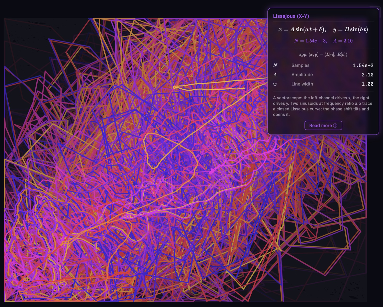
x = A·sin(at + δ), y = B·sin(bt) in the corner tile.
Take away the time axis, feed one signal into the horizontal and another into the vertical, and the moving dot stops drawing a graph and starts drawing a figure. Spiralyst Lab plots the left audio channel against the right, so two related tones trace a stable looping curve whose shape reveals their frequency ratio and the phase between them.
The textbook Lissajous figure is what you get when both signals are sinusoids:
$$x = A\sin(at + \delta),\quad y = B\sin(bt)$$
The frequency ratio \(a/b\) sets which figure appears — an ellipse for 1:1, a figure-eight for 1:2, ever more elaborate knots and ribbons as the ratio grows. The phase offset \(\delta\) tilts and opens the figure. In the app the axes are simply the L and R audio channels:
$$(x, y) = (L[n],\, R[n])$$
which makes it a true vectorscope. A mono signal collapses to a single diagonal line; a wide stereo mix blooms into a cloud; a channel flipped out of phase swings to the opposite diagonal — an instant read on whether the mix will survive being summed to mono. That's genuinely useful in mastering, not just decoration.
Controls: Live monitor, Auto-gain, Samples (the trail length), Line width, Amplitude.
Spectrum — the frequency analyzer
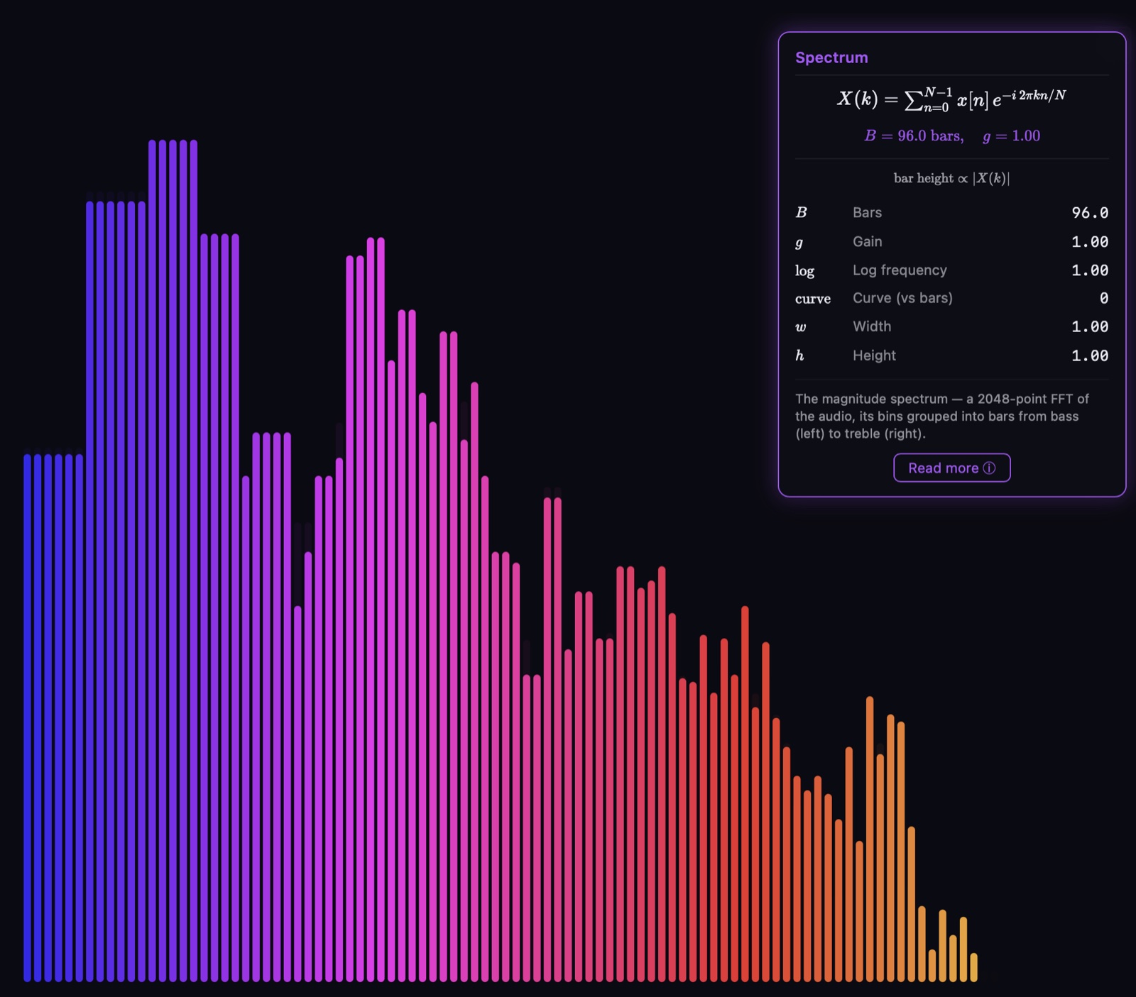
X(k) = Σ x[n] · e^(−i·2πkn/N) pinned in the corner tile.
Where the oscilloscope shows sound in time, the spectrum shows it in frequency. It breaks the incoming waveform into its constituent sine waves and draws a bar (or a curve) whose height is the energy at each pitch. Deep bass on the left, bright treble on the right.
The transform underneath is the discrete Fourier transform:
$$X(k) = \sum_{n=0}^{N-1} x[n]\cdot e^{-i\,2\pi k n / N}$$
It projects a block of \(N\) time samples onto sinusoids and returns one complex number \(X(k)\) per frequency bin \(k\). The bar height is the magnitude \(|X(k)|\) — how much energy the signal carries at that frequency. Phase is discarded; only loudness per pitch is shown.
The Log frequency control switches the bar layout from evenly spaced bins to logarithmically spaced ones, so each octave occupies the same horizontal width — the way the ear hears it. (Your cochlea is a coiled biological spectrum analyzer, its hair cells tuned from low pitches at one end to high at the other, so a log-frequency display is a closer match to your own hearing.) Spiralyst Lab's spectrum mode is the same frequency data that drives the audio-reactive fractals — drawn visibly, with no added audio cost.
Controls: Live monitor, Auto-gain, Bars (32–256), Curve (vs bars), Log frequency, Gain, Width, Height.
Harmonograph — the Victorian pendulum's drawing
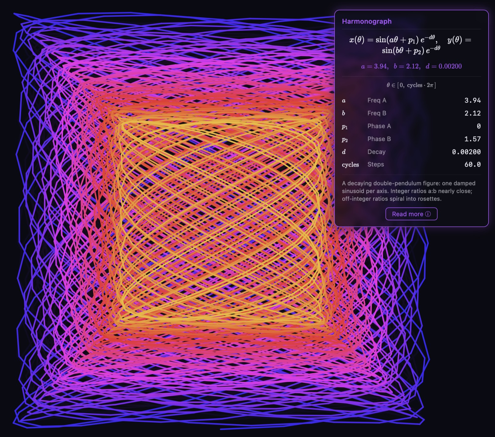
x(θ) = sin(aθ + p₁)·e^(−dθ), y(θ) = sin(bθ + p₂)·e^(−dθ) pinned in
the corner tile.
The fourth scope is the one with no microphone in it. The harmonograph is a Victorian parlor wonder — a table-sized contraption of swinging pendulums linked to a pen, left to draw on its own. Two pendulums swing at slightly different frequencies, the pen weaves an intricate figure, and as friction bleeds the swings of their energy, the figure spirals gently inward to a still point.
Spiralyst Lab traces the figure parametrically:
$$x(\theta) = \sin(a\theta + p_1)\cdot e^{-d\theta},\quad y(\theta) = \sin(b\theta + p_2)\cdot e^{-d\theta}$$
for \(\theta \in [0,\, \text{cycles}\cdot 2\pi]\). The frequency ratio \(a/b\) sets the figure; integer ratios make nearly-closed curves and off-integer ratios spiral into rosettes. The decay constant \(d\) controls how fast the swing winds inward. Phases \(p_1\) and \(p_2\) rotate the figure and open it.
An honest note: this is a mathematical recreation — a single damped sinusoid per axis — not a simulation of a real multi-pendulum harmonograph rig. The essential motion is captured, not the physics of swinging masses on coupled hinges.
Although the harmonograph has no audio in its draw, every one of its sliders is audio-bindable through the regular animator, and a Live monitor toggle wires Freq A and Freq B to bass and treble amplitude so the figure morphs between integer ratios as the music plays. A mathematical pendulum that dances to a track.
Controls: Live monitor, Freq A (1–8), Freq B (1–8), Phase A (0–π), Phase B (0–π), Decay (0–0.01), Steps (10–200). No Auto-gain — it's parametric, not amplitude-scaled.
How scopes fit with the rest of the studio
A scope is a render type, sitting in the type dropdown alongside the 27 fractals under its own Scopes group. That means it inherits everything the studio already does:
- Same color and effects controls — hue range, palette, glow, trails, vignette, background gradient. Style a scope to match a brand or a stage.
- Same audio reactivity — every slider on every scope can be bound to a frequency band, the same way fractal sliders are. (The audio-driven scopes already react in real time; the binding lets you also breathe their parameters with the music.)
- Same recording and export — File → Record Video captures scopes the same way it captures fractals. Save a 10-second waveform loop as MP4 for a release reel.
- Full Math Mode coverage — every scope has the live formula tile, the textbook-depth info card, the hero formula, and the per-slider guide (see the Math Mode page). All 27 fractals and all 4 scopes carry the same overlay.
- Same system-audio capture — no virtual audio cables, no loopback drivers. The oscilloscope, Lissajous, and spectrum modes read the live tap directly.
Use it in a classroom
A few starting points for educators.
Pre-algebra — graphs from the world. Open the oscilloscope and play any sound. The waveform is a graph: the horizontal axis is time, the vertical axis is amplitude, the curve is the function. Watch a sustained note (a pure-ish whistled tone, say) and the curve is nearly periodic. Watch a drum and it's a sharp transient. The same xy-axes a class draws on paper, rendered live.
High-school physics — phase and superposition. Switch to Lissajous and play two pure tones at known frequencies. A 1:1 ratio with zero phase is a diagonal line; a 1:1 ratio with quarter-cycle phase is a circle; the same circle going the other way around is the opposite quarter-cycle. The same picture every physics textbook draws to explain phase, rendered from real audio.
Calculus / signals — Fourier in real time. Switch to the spectrum. Play any single instrument and the bars cluster at the fundamental and its harmonics; play a full mix and the energy spreads across the spectrum. Fourier's claim — that any signal is a sum of sines — is just a fact written on the screen.
Math history / curiosity — the Victorian parlor. Open the harmonograph and step the frequency ratio from 1:1 to 1:2 to 2:3 to 3:5 to a deeply irrational pair. Closed figures, then nearly-closed, then rosettes, then a slow irrational drift. The same pictures Victorian parlor guests watched a real pendulum rig draw, computed from the same essential math.
An ECG (electrocardiogram) is essentially a specialized oscilloscope: it traces the heart's electrical waveform the same way this one traces sound. That's the same instrument that shows you a kick drum's transient and a cardiologist a patient's rhythm. Useful framing in a biology or pre-med class.
Use it as a hobbyist or an audio engineer
Outside the classroom, scopes have practical lives.
- The oscilloscope as a listening companion. Leave it running with an album playing. Loud passages fill the vertical space, quiet ones shrink to a thread, a drum hit spikes and decays, a sustained chord settles into a rich repeating shape. The shape of every sound, while you listen to it.
- The Lissajous as a stereo meter. Drop the X-Y view onto a mix and check the picture. A wide cloud means a wide stereo image; a tight diagonal line means it has collapsed toward mono; a swing to the opposite diagonal means something is out of phase. This is genuinely how mastering engineers check mono-compatibility, and the same display works inside Spiralyst Lab on whatever your Mac is playing.
- The spectrum as the always-on analyzer. If you're tuning a mix or learning a song, having the spectrum visible while you listen is the audio equivalent of running a syntax-highlighter while you read code. Bass build-up shows; harshness in the upper mids shows; a missing midrange shows. Same data the studio's reactive fractals are reading, just drawn.
- The harmonograph as the math toy. If you grew up with a Spirograph set, you already know the harmonograph — its geared, pocket-sized descendant. Sliding the frequency ratios, phases, and decay is hours of exploration before any of it touches a beat. And when you do bind it to audio, the figure dances to the track.
And because scopes inherit File → Record Video, a 10-second Lissajous loop with a track playing makes a perfect square Instagram clip. A spectrum reel for the release graphic. The waveform of a drop, for an EPK.
Privacy and offline use
Scopes work exactly the same way the rest of Spiralyst Lab does. The audio is captured live on your Mac and analyzed in the moment, never recorded or transmitted. There is no telemetry, no external network, no account. Turning on a scope doesn't change what data Spiralyst Lab collects, because Spiralyst Lab doesn't collect data. Read the privacy promise for the rest of the story.
Where to go from here
- Browse the gallery — once scope captures land you'll find each of the four modes there, with the same prose this page summarises. (Coming with the v3.2.0 release.)
- Read the Scopes release post for the launch announcement and in-context demos.
- See the Math Mode page — every scope has the same live-formula overlay as the 27 fractals.
- Get Spiralyst Lab if you don't have it yet — $24.99 for a one-year license, direct download. Scopes ship in v3.2.0.
Get Spiralyst Lab — $24.99/yr ← Back to Support
Math typesetting on this page is rendered by KaTeX 0.17.0 (MIT).